GGCE-PETSc interface: introduction
In this tutorial, we show how to use GGCE’s interface with PETSc for those massively parallel calculations involving very large sparse matrices. We do this on the example of calculating the spectral function near the polaron band in the Holstein model.
What is PETSc?
The basic functionality of GGCE-PETSc is easily accessible once PETSc has been installed following the instructions in the Installation section. As explained in the install notes, PETSc is a purpose-built library for linear algebra that allows MPI-parallel operations. This enables PETSc to tackle extremely large matrices, the only limitation being the available resources.
The reason this is useful in GGCE is that for large enough cloud configurations, and especially in higher dimensions (which will be available in future versions of GGCE) and at finite temperature (see Finite-temperature calculations), applying the method can result in large sparse matrices with dimensions in the hundreds of thousands or even millions. Standard techniques for solving such systems, even threaded ones like those available in SciPy, cannot handle such matrices due to memory and/or time constraints.
PETSc comes equipped with methods for constructing MPI-shareable data structures for matrices and solution vectors, as well as a great variety of “solvers” (called contexts) for solving them. These solvers are able to make use of the MPI-shared data layout to a) reduce memory load on any one process, and b) speed-up the computation by exploiting known parallelization schemes.
How do we access PETSc in GGCE?
PETSc has a Python API (petsc4py) that wraps most of PETSc’s functionality for
convenient access in Python. The GGCE-PETSc interface is built using those wrappers.
Currently implemented is the MUMPS
context of PETSc. MUMPS (Multifrontal Massively Parallel sparse direct Solver) is a
free, MPI-enabled, well-tested and reliable direct sparse matrix solver
often used in situations involving big matrices, such as in finite-element
modelling (FEM). MUMPS is available in GGCE as the MassSolverMUMPS Solver
object (through PETSc). The object implements all the same methods as a standard
GGCE Solver object, including a parallel-enabled .greens_function(),
and can be used in exactly the same way as a parallel GGCE solver – by passing in
the MPI communicator and executing the script with mpirun or mpiexec.
After the simple import command
from ggce.executors.petsc4py import MassSolverMUMPS
from mpi4py import MPI
we may use the usual GGCE syntax to set up a quick calculation
model = Model.from_parameters(hopping=1.)
model.add_(
          "Holstein",
          phonon_frequency=1.,
          phonon_extent=2,
          phonon_number=8,
          dimensionless_coupling_strength=0.0
          )

system = System(model)

COMM = MPI.COMM_WORLD
solver = MassSolverMUMPS(system=system, mpi_comm=COMM)
Polaron dispersion
Now for some physics. In the Holstein model with dimensionless coupling \(\lambda = g^2 / 2\Omega t\) and (Einstein) phonon frequency \(\Omega\), we expect the polaron band to be roughly \(E_P(k=0) \approx -2t - \lambda\), and increase in energy away from \(k=0\). Fixing \(\Omega = 1, \lambda = 0.5\), this implies we should investigate a range of \(\omega \in [-3, -1]\) to get a good view of the polaron band across the Brillouin zone.
kgrid = np.linspace(0, np.pi, 100)
wgrid = np.linspace(-3., -1., 200)

COMM = MPI.COMM_WORLD
solver = MassSolverMUMPS(system=system, mpi_comm=COMM)
G = solver.greens_function(kgrid, wgrid, eta=0.05, pbar=True)
The result can be plotted with pcolormesh – note that the G array of Green’s
functions needs to be transposed to correspond to the “normal” alignment of
\(k,\omega\).
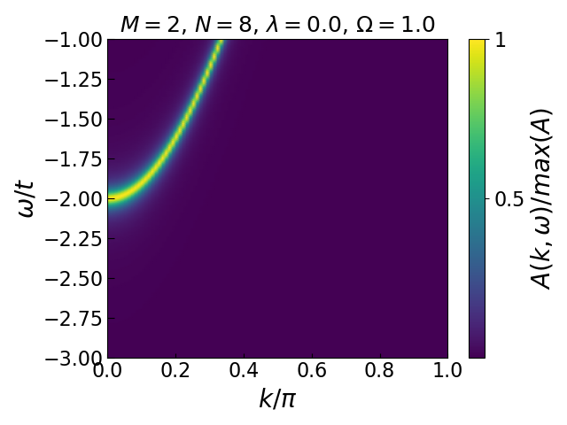
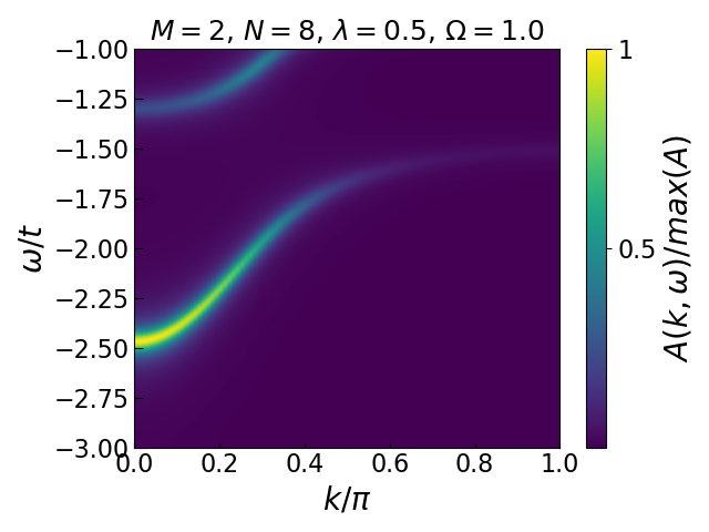
On the left we show the electronic band of the noninteracting system, for reference. As we can see, adding a Holstein interaction term to the Hamiltonian results in the lowering of the electron’s energy (shifting of the band down), as well as changing its hopping behaviour (dispersion).
Visually, you can tell that the band curvature around the \(k=0\) point is changed – the band is flattened in that neighbourhood. A flattened band means a higher effective mass and thus a “slower” electron. This makes sense: the cloud of phonons that the electron is now forced to drag around is slowing it down, making it move as if through molasses.
This concludes an introduction to the basic features of the GGCE-PETSc interface. To learn more about some of the advanced features on offer, see GGCE-PETSc interface: advanced features.