Benchmarking GGCE
In this tutorial, we will show GGCE in operation. Specifically, we will
demonstrate how the objects you learned about in the previous section –
Model, System, and Solver – can be used to produce a spectral
function \(A(k,\omega)\).
To benchmark GGCE, we will compare our result against a prior numerical study (Berciu & Fehske, PRB 82, 085116 (2010)). In that study, the authors employed the momentum average approximation (MA) – a technique from which GGCE directly descends – to calculate the spectrum of the Edwards Fermion Boson model we introduced in the previous tutorial.
As a first sanity check, we will compare GGCE to its ancestor.
Step 1: prepare the calculation
In the reference paper linked above, a single-particle Green’s function and spectrum are calculated for the Edwards Fermion Boson coupling Hamiltonian,
For the purposes of this demonstration, it is not important what this model represents: as long as it can be expressed in terms of creation/annihilation operators \(b_j^\dagger, b_j, c_j^\dagger, c_j\), GGCE can give us its spectrum (but see the note below for some physical intuition for the model).
Note
An intuitive picture for this model of coupling is the following: every time a fermion hops to a site j with no bosons, it leaves behind a boson excitation created by \(b^\dagger_j\). On the other hand, if the fermion hops to a site where a boson already exists, the boson gets destroyed by \(b_i\).
This might seem like a strange model at first glance. However, taking fermions to be holes and the bosonic excitations to be “spin-flips”, or magnons, this model allows one to “mimic the motion” of a charge carrier “through an antiferromagnetically ordered spin background”, such as thought to be relevant in the context of cuprate CuO layers. See Sec. II in Berciu & Fehske, PRB 82, 085116 (2010) for more details.
The Model can be initialized as before
from ggce import Model
model = Model.from_parameters(hopping=0.1)
model.add_(
    "EdwardsFermionBoson",
    phonon_frequency=1.25,
    phonon_extent=3,
    phonon_number=9,
    dimensionless_coupling_strength=2.5
)
Here we specifically picked model parameters corresponding to those used in Fig. 5 (top panel) from the reference paper.
Note
While the phonon_number is not set explicitly in the reference,
in MA it is understood that it is varied until physical results,
such as spectra, are converged with respect to it. Here we found the value
phonon_number = 9 resulted in appropriate convergence. In general,
a full convergence study in all variational parameters should be conducted
to make sure convergence is reached.
Creating the System, we optionally choose to pass the option
autoprime=False. This defers the building of the system of
equations within System until we instantiate a Solver.
from ggce import System
system = System(model, autoprime=False)
Note
In a large variational calculation, the creation – or “priming” –
of the System object can take a long time.
Passing autoprime=False allows us to practice “lazy computation”:
we can symbolically create the System object, adjust its parameters
later on and do other things in the script. We defer the construction
of the system of equations (stored as attributes of the System
class) until actual computation of the spectrum begins – i.e.
until a Solver based on this System is initialized.
Step 2: obtain the spectrum
This time, let’s use a sparse solver to obtain the spectrum. Syntactically,
the differences from using a dense solver are minimal: we simply use a
different class SparseSolver
from ggce import SparseSolver
solver = SparseSolver(system)
The SparseSolver class, which relies on SciPy’s sparse matrix format
and solvers, can be helpful in the case of large variational calculations
where memory constraints become significant and prevent us from using the
continued fraction, dense solver approach.
Using the sparse format to store the matrix results in significant memory
savings and also allows partial threaded parallelization. This happens
internally in SciPy and it controlled by setting the environment variable
OMP_NUM_THREADS if your NumPy is compiled with default BLAS/LAPACK or
OpenBLAS, and with MKL_NUM_THREADS if your NumPy relies on the MKL backend.
To set this variable and have it automatically be detected by NumPy, issue the following command in the same terminal you are using to run this code (Unix) to (for example) run all subsequent GGCE calculations on 2 cores
export OMP_NUM_THREADS=2
(On Windows, you can either find an equivalent command to set this in the shell, or set it globally through the Control Panel.)
Note
The sparse matrix approach exploits the fact that the System-provided
matrix is quite sparse, owing to the “local” nature of many Hamiltonians
of interest in condensed matter and specifically of the electron-phonon
coupling.
By “local” we mean that typically in a tight-binding model, only “close neighbour” hoppings are included. While one can have quite large neighbour shells, this is still a far cry from a model with all-to-all hopping. A similar comment can be made about interactions, which are usualy considered to be on-site or between neighbours, but rarely all-to-all (although see the SYK model). This means matrices representing Hamiltonians are necessarily at least somewhat sparse.
Finally, we solve the system and plot the result against the reference.
k = np.array([0.0])
w = np.linspace(-3.0, -1.0, 100)
G = solver.greens_function(k, w, eta=0.005, pbar=True)
A = -G.imag / np.pi
We can plot the results directly against the literature data as a comparison.
Note that the option pbar=True activates a visual progress bar (powered
by tqdm) that helps track the progress of the spectrum calculation.
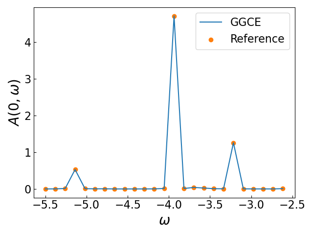
As we can see, the GGCE results match the reference very well.
The .greens_function() method is merely a convenient wrapper for .solve()
that can execute a loop over two arrays, of momentum \(k\) and frequency
\(\omega\). You could achieve the same functionality by writing your own
loop: symbolically
for k, w in zip(kgrid, wgrid):
  Green_Funcs[i,j] = solver.solve(k, w, eta)
However, .greens_function() has the advantage that it has built-in parallelizability.
If you have mpi4py installed and properly configured, you can run .greens_function()
on your chosen \(k,\omega\) arrays and they will be automatically partitioned
between the MPI ranks, no work required!
See the next tutorial Running GGCE in parallel where we show how to use GGCE with MPI parallelization.